library(here)
library(tidyverse)
library(janitor)
library(ggplot2)
library(recipes)
library(xgboost)
library(beepr)Ocean acidification, driven primarily by human-induced carbon emissions, already poses a huge problem for our oceans, economy, and well being. For proper ecosystem management, is important to understand which areas of the ocean are at higher risk. This workbook uses machine learning techniques to accurately predict ocean acidification to aid in management.
What is Ocean Acidification?
Our oceans absorb about 30% of the CO2 in our atmosphere. So, as CO2 emissions increase, CO2 in our oceans does, as well. This may not sound like a problem, but CO2 quickly breaks down and creates acid that disintegrates things like sea shells and coral reefs that fish, shellfish, and ultimately, humans, depend on. (“What Is Ocean Acidification?” 2023) More than 3 billion people around the world rely on food from our oceans(“A Healthy Ocean Depends on Sustainably Managed Fisheries” 2021), and ocean acidification poses a huge risk to the availability of the food.
Kaggle Competition Background
The California Cooperative Oceanic Fisheries Investigations (CalCOFI for short) studies marine ecosystems across California to help drive sustainable environmental management in the context of climate change.(“About CalCOFI,” n.d.) In March of 2023, CalCOFI partnered with the Bren School at UC Santa Barbara to search for an effective predictive model for ocean acidification. As part of my Environmental Data Science class, “Machine Learning in Environmental Science”, us master’s students had all entered the Kaggle competition to find the best predictive machine learning model given the data available1. The prize? CalCOFI swag (and helping sustainable ecosystem management).
The Winning Competition Code
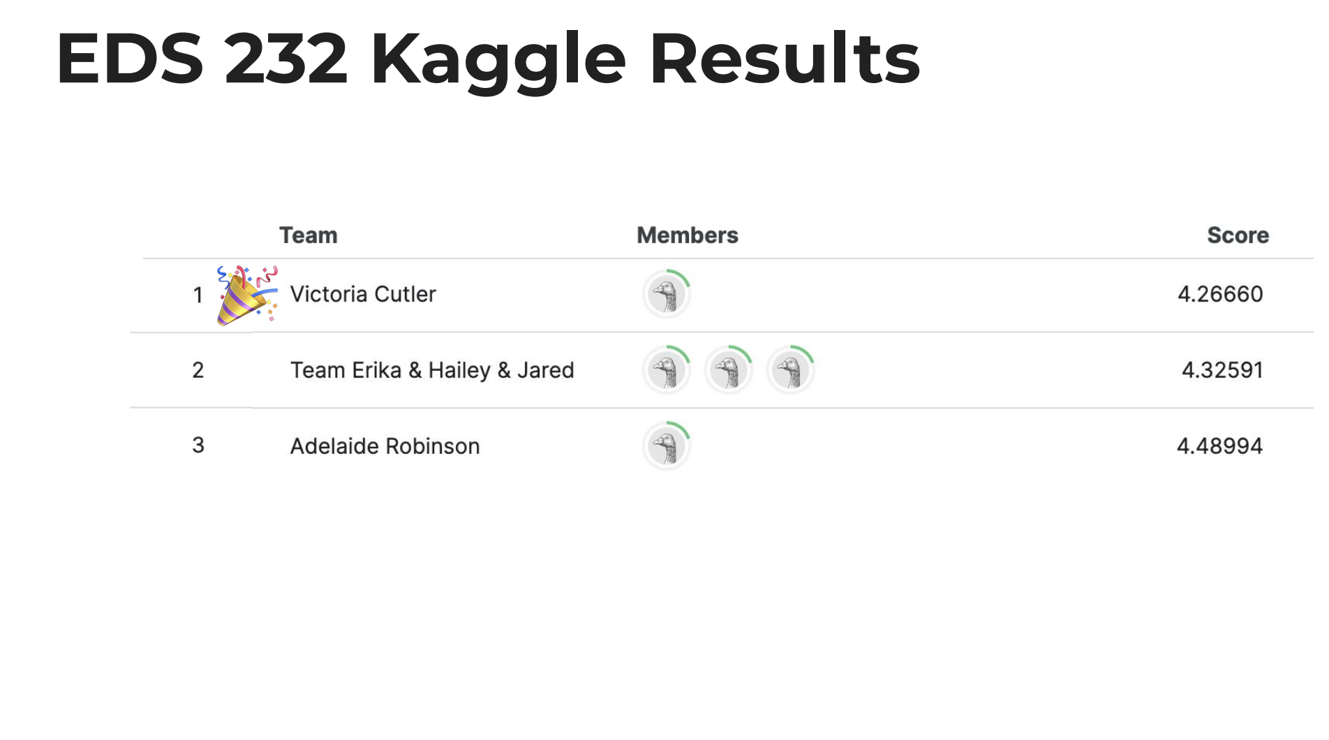
Yes, I won. Don’t be so shocked. And yes, I got a lot of swag! Please read on, below, for not just the code but also my thought process a long the way.
Load Libraries
Load and Clean Data
Here I load in the training and testing data (already pre-split to ensure consistency in competition assessment). I then correct any data quality issues. It turned out that the training and testing data had a couple inconsistencies, so I fixed those up and removed any unnecessary columns.
# storing file paths
train_file_path <- here("posts","predicting-ocean-acidification","data", "train.csv")
test_file_path <- here("posts","predicting-ocean-acidification","data", "test.csv")

# reading in data

  # raw training data
train_raw <- read_csv(file = train_file_path) |>
  clean_names() |>
  glimpse()
Rows: 1,454
Columns: 19
$ id <dbl> 1, 2, 3, 4, 5, 6, 7, 8, 9, 10, 11, 12, 13, 14, 15, 1…
$ lat_dec <dbl> 34.38503, 31.41833, 34.38503, 33.48258, 31.41432, 32…
$ lon_dec <dbl> -120.6655, -121.9983, -120.6655, -122.5331, -121.997…
$ no2u_m <dbl> 0.030, 0.000, 0.180, 0.013, 0.000, 0.080, 0.007, 0.0…
$ no3u_m <dbl> 33.80, 34.70, 14.20, 29.67, 33.10, 5.00, 38.76, 0.10…
$ nh3u_m <dbl> 0.00, 0.00, 0.00, 0.01, 0.05, 0.14, 0.00, 0.05, 0.03…
$ r_temp <dbl> 7.79, 7.12, 11.68, 8.33, 7.53, 13.05, 6.31, 19.28, 7…
$ r_depth <dbl> 323, 323, 50, 232, 323, 50, 518, 2, 323, 170, 30, 23…
$ r_sal <dbl> 141.2, 140.8, 246.8, 158.5, 143.4, 293.1, 114.6, 403…
$ r_dynht <dbl> 0.642, 0.767, 0.144, 0.562, 0.740, 0.176, 0.857, 0.0…
$ r_nuts <dbl> 0.00, 0.00, 0.00, 0.01, 0.05, 0.14, 0.00, 0.05, 0.03…
$ r_oxy_micromol_kg <dbl> 37.40948, 64.81441, 180.29150, 89.62595, 60.03062, 2…
$ x13 <lgl> NA, NA, NA, NA, NA, NA, NA, NA, NA, NA, NA, NA, NA, …
$ po4u_m <dbl> 2.77, 2.57, 1.29, 2.27, 2.53, 0.75, 3.16, 0.19, 2.63…
$ si_o3u_m <dbl> 53.86, 52.50, 13.01, 38.98, 49.28, 5.90, 76.82, 0.17…
$ ta1_x <dbl> 2287.45, 2279.10, 2230.80, 2265.85, 2278.49, 2219.87…
$ salinity1 <dbl> 34.1980, 34.0740, 33.5370, 34.0480, 34.1170, 33.2479…
$ temperature_deg_c <dbl> 7.82, 7.15, 11.68, 8.36, 7.57, 13.06, 6.36, 19.28, 7…
$ dic <dbl> 2270.170, 2254.100, 2111.040, 2223.410, 2252.620, 20… # raw testing data
test_raw <- read_csv(file = test_file_path) |>
clean_names() |>
glimpse()Rows: 485
Columns: 17
$ id <dbl> 1455, 1456, 1457, 1458, 1459, 1460, 1461, 1462, 1463…
$ lat_dec <dbl> 34.32167, 34.27500, 34.27500, 33.82833, 33.82833, 33…
$ lon_dec <dbl> -120.8117, -120.0333, -120.0333, -118.6250, -118.625…
$ no2u_m <dbl> 0.02, 0.00, 0.00, 0.00, 0.02, 0.17, 0.00, 0.00, 0.00…
$ no3u_m <dbl> 24.0, 25.1, 31.9, 0.0, 19.7, 4.2, 21.5, 26.1, 31.9, …
$ nh3u_m <dbl> 0.41, 0.00, 0.00, 0.20, 0.00, 0.10, 0.00, 0.01, 0.00…
$ r_temp <dbl> 9.51, 9.84, 6.60, 19.21, 10.65, 12.99, 10.29, 9.50, …
$ r_depth <dbl> 101, 102, 514, 1, 100, 19, 99, 169, 319, 523, 101, 5…
$ r_sal <dbl> 189.9, 185.2, 124.1, 408.1, 215.5, 284.9, 207.3, 173…
$ r_dynht <dbl> 0.258, 0.264, 0.874, 0.004, 0.274, 0.075, 0.266, 0.3…
$ r_nuts <dbl> 0.41, 0.00, 0.00, 0.20, 0.00, 0.10, 0.00, 0.01, 0.00…
$ r_oxy_micromol_kg <dbl> 138.838300, 102.709200, 2.174548, 258.674300, 145.83…
$ po4u_m <dbl> 1.85, 2.06, 3.40, 0.27, 1.64, 0.65, 1.77, 2.17, 2.78…
$ si_o3u_m <dbl> 25.5, 28.3, 88.1, 2.5, 19.4, 5.4, 21.8, 31.5, 48.6, …
$ ta1 <dbl> 2244.94, 2253.27, 2316.95, 2240.49, 2238.30, 2224.99…
$ salinity1 <dbl> 33.8300, 33.9630, 34.2410, 33.4650, 33.7200, 33.3310…
$ temperature_deg_c <dbl> 9.52, 9.85, 6.65, 19.21, 10.66, 12.99, 10.30, 9.52, …# looking at data frame similarities / differences
colnames_df1 <- colnames(train_raw)
colnames_df2 <- colnames(test_raw)
# common columns
common_cols <- intersect(colnames_df1, colnames_df2)
common_cols [1] "id" "lat_dec" "lon_dec"
[4] "no2u_m" "no3u_m" "nh3u_m"
[7] "r_temp" "r_depth" "r_sal"
[10] "r_dynht" "r_nuts" "r_oxy_micromol_kg"
[13] "po4u_m" "si_o3u_m" "salinity1"
[16] "temperature_deg_c" # looking for different columns between the training and testing data
unique_cols_df1 <- setdiff(colnames_df1, common_cols)
unique_cols_df1[1] "x13" "ta1_x" "dic" unique_cols_df2 <- setdiff(colnames_df2, common_cols)
unique_cols_df2[1] "ta1"# adjusting training data per column naming differences
train_data <- train_raw |>
select(-x13) |> # removing since all NULL
rename(ta1 = ta1_x) # changing the name to match the test_raw namingData Exploration for Machine Learning Algorithm Selection
Below I create a full data set with both the training and testing data. I then explore data distributions for each of the features since this will inform the machine learning algorithm I select for ocean acidification prediction.
# adding all the data together to plot data distributions for each variable. This is to check variance and outliers to inform which ML algorithm to use
full_data <- train_data |>
  select(-dic) |> # removing the dic variable we're predicting since the test data doesn't have this variable and i don't want to look at the data distribution in case leaving out the test data introduces bias
  rbind(test_raw)

# histograms to explore data distributions and look at variance/outliers
ggplot(data = full_data, aes(x = no2u_m)) +
  geom_histogram()
`stat_bin()` using `bins = 30`. Pick better value with `binwidth`.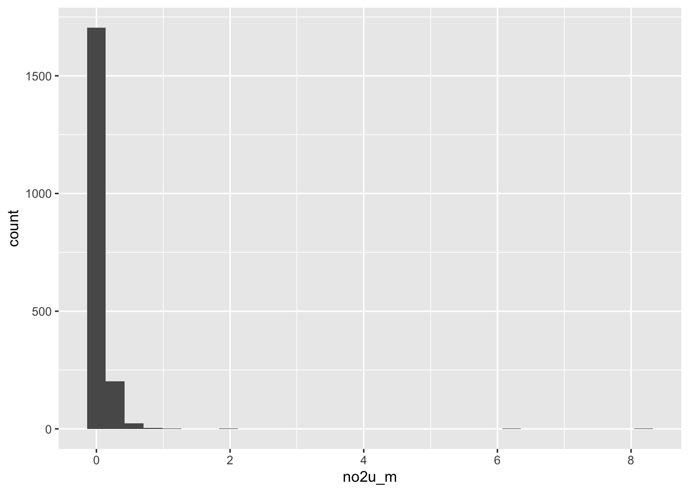
ggplot(data = full_data, aes(x = no3u_m)) +
  geom_histogram()
`stat_bin()` using `bins = 30`. Pick better value with `binwidth`.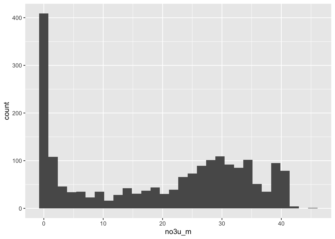
ggplot(data = full_data, aes(x = nh3u_m)) +
  geom_histogram() # potential outliers here
`stat_bin()` using `bins = 30`. Pick better value with `binwidth`.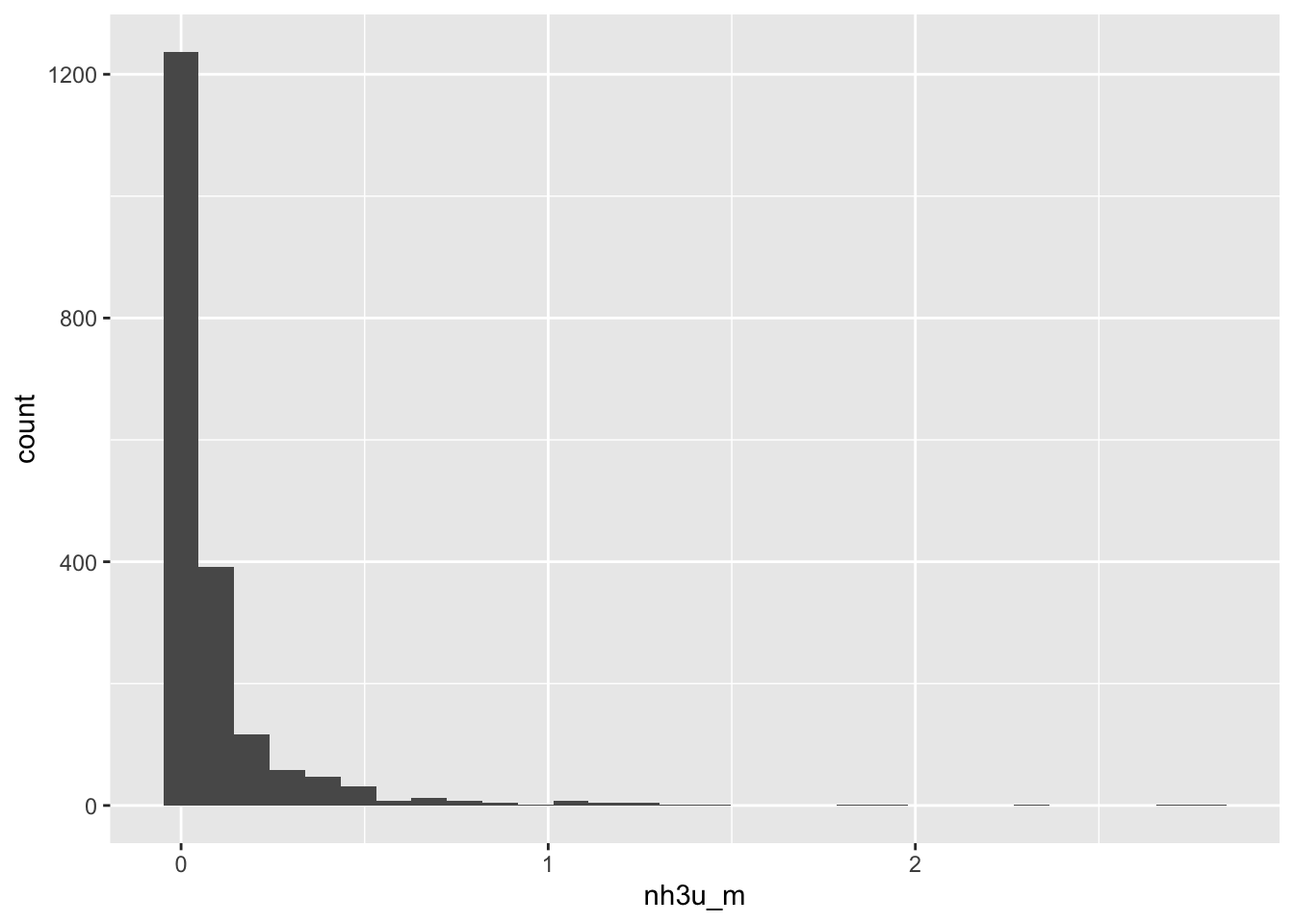
ggplot(data = full_data, aes(x = r_temp)) +
  geom_histogram()
`stat_bin()` using `bins = 30`. Pick better value with `binwidth`.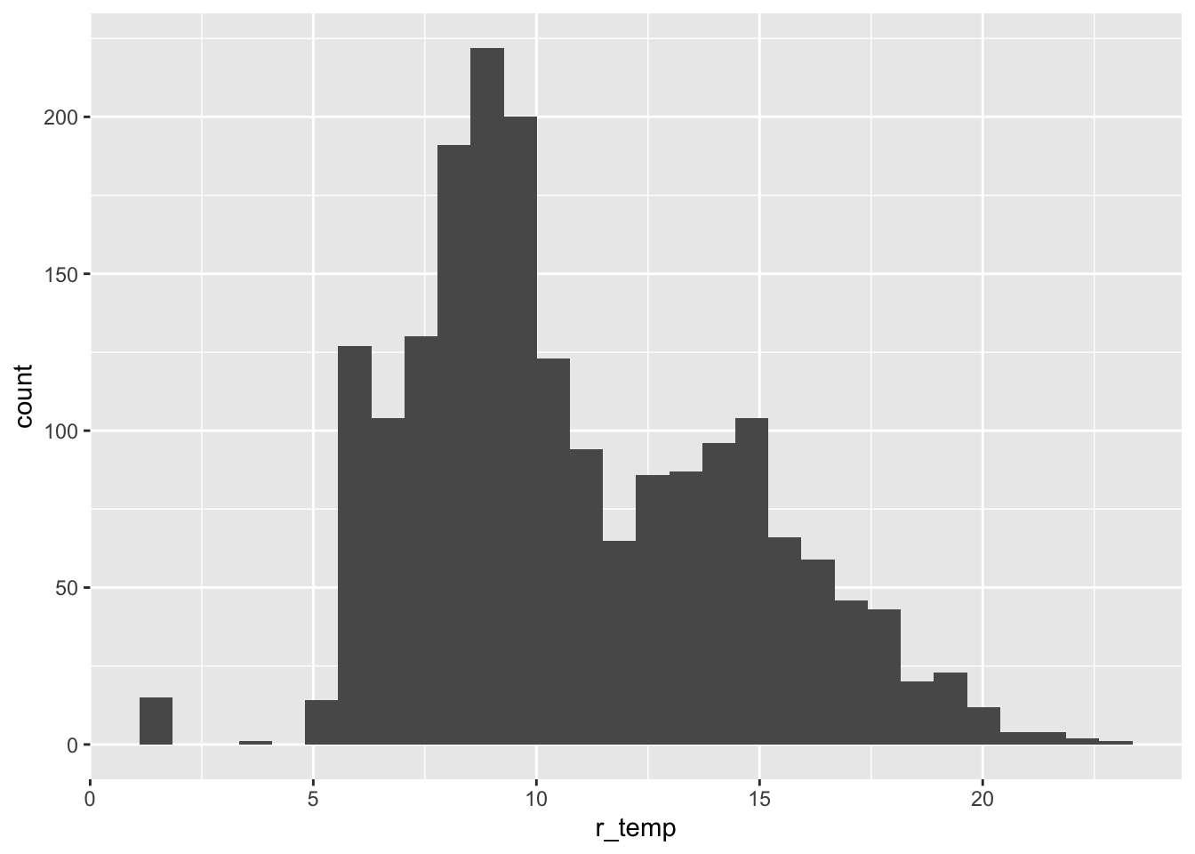
ggplot(data = full_data, aes(x = r_depth)) +
  geom_histogram() # potential outliers here:
`stat_bin()` using `bins = 30`. Pick better value with `binwidth`.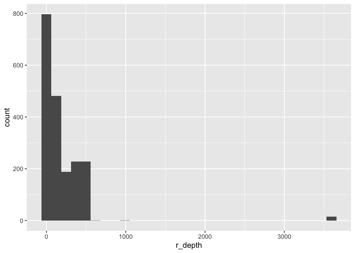
ggplot(data = full_data, aes(x = r_sal)) +
  geom_histogram()
`stat_bin()` using `bins = 30`. Pick better value with `binwidth`.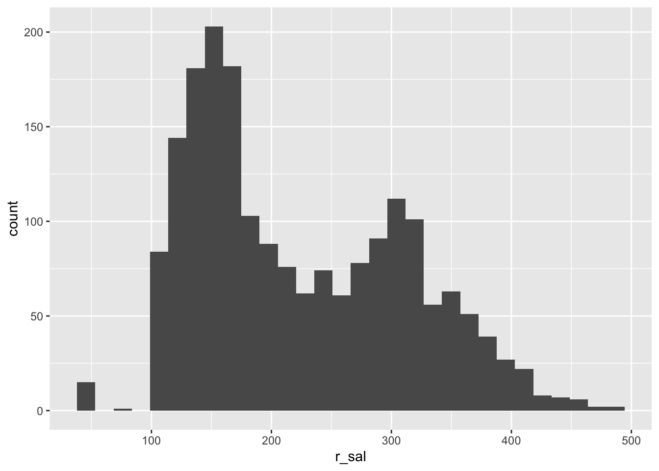
ggplot(data = full_data, aes(x = r_dynht)) +
  geom_histogram() # potential outliers here
`stat_bin()` using `bins = 30`. Pick better value with `binwidth`.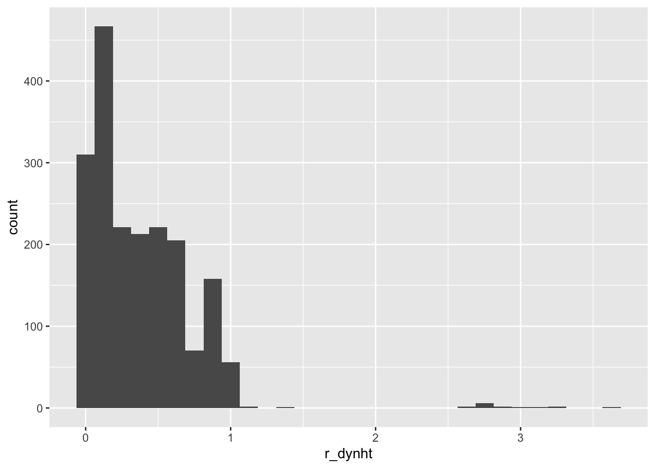
ggplot(data = full_data, aes(x = r_nuts)) +
  geom_histogram() # potential outliers here
`stat_bin()` using `bins = 30`. Pick better value with `binwidth`.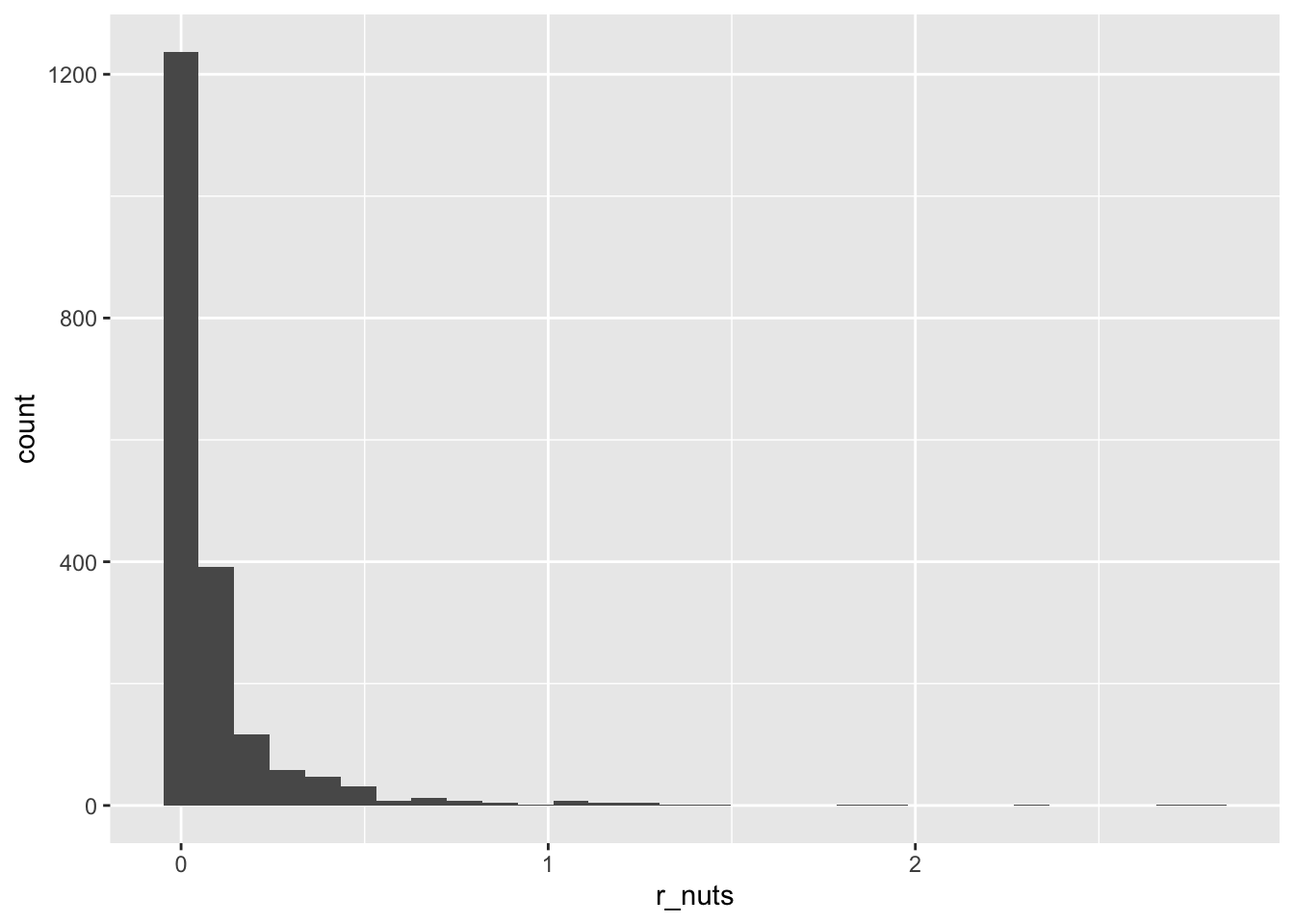
XGBoost Model
After plotting the data distributions, I see a lot of outliers. I also know that I can’t use a classification algorithm since my prediction variable is continuous. I choose to build an extreme gradient boosted treet (XGBoost) machine learning algorithm to build my ocean acidification prediction model. I use this algorithm since gradient boosted models, if properly tuned, can be the most flexible and accurate predictive models. I choose an extreme gradient boosted model since it can handle outliers well and has many hyperparameters that reduce overfitting.
Recipe
# using the xgboost model since this is a powerful ML algorithm that can handle outliers. Code is adapted from: https://bradleyboehmke.github.io/HOML/gbm.html

  # recipe
xgb_prep <- recipe(dic ~ ., data = train_data) %>% # using all features for predicting dic (ocean acidification)
  prep(training = train_data, retain = TRUE) %>%
  juice()

  # separating data used for predictions from the predicted values
X <- as.matrix(xgb_prep[setdiff(names(xgb_prep), "dic")])
Y <- xgb_prep$dic
Hyperparameter Tuning and Model Fit Assessment
# set seed for reproducibility
set.seed(123)

# creating a hyperparameter grid for all xgboost hyperparameters
hyper_grid <- expand.grid(
  eta = 0.01,
  max_depth = 3,
  min_child_weight = 3,
  subsample = 0.5,
  colsample_bytree = 0.5,
  gamma = c(0, 1, 10, 100, 1000),
  lambda = c(0, 1e-2, 0.1, 1, 100, 1000, 10000),
  alpha = c(0, 1e-2, 0.1, 1, 100, 1000, 10000),
  rmse = 0,          # a place to dump RMSE results
  trees = 0          # a place to dump required number of trees
)

# loop to search through the grid and apply hyperparameters to all 10 cv folds
for(i in seq_len(nrow(hyper_grid))) {
  set.seed(123)
  m <- xgb.cv(
    data = X,
    label = Y,
    nrounds = 4000,
    objective = "reg:squarederror",
    early_stopping_rounds = 50,
    nfold = 10,
    verbose = 0,
    params = list(
      eta = hyper_grid$eta[i],
      max_depth = hyper_grid$max_depth[i],
      min_child_weight = hyper_grid$min_child_weight[i],
      subsample = hyper_grid$subsample[i],
      colsample_bytree = hyper_grid$colsample_bytree[i],
      gamma = hyper_grid$gamma[i],
      lambda = hyper_grid$lambda[i],
      alpha = hyper_grid$alpha[i]
    )
  )
  hyper_grid$rmse[i] <- min(m$evaluation_log$test_rmse_mean)
  hyper_grid$trees[i] <- m$best_iteration
}

# store results where rmse is greater than 0
rmse_hp_results <- hyper_grid %>%
  filter(rmse > 0) %>%
  arrange(rmse)

# store the best hyperparameters
best_eta <- rmse_hp_results$eta[1]
best_md <- rmse_hp_results$max_depth[1]
best_cw <- rmse_hp_results$min_child_weight[1]
best_ss <- rmse_hp_results$subsample[1]
best_csbt <- rmse_hp_results$colsample_bytree[1]
best_g <- rmse_hp_results$gamma[1]
best_l <- rmse_hp_results$lambda[1]
best_a <- rmse_hp_results$alpha[1]

# beep when process is done since this process can take hours
beep()
Training the Training Data Based on Optimal Hyperparameters
# optimal parameter list
params <- list(
  eta = best_eta,
  max_depth = best_md,
  min_child_weight = best_cw,
  subsample = best_ss,
  colsample_bytree = best_csbt,
  gamma = best_g,
  lambda = best_l,
  alpha = best_a
)

# train the model on the training data given these optimal parameters
xgb.fit.final <- xgboost(
  params = params,
  data = X,
  label = Y,
  nrounds = 3944,
  objective = "reg:squarederror",
  verbose = 0
)
Predicting the Test Data Set Ocean Acidification for Competition Assessment
# predict on the test data set
X_test <- as.matrix(test_raw)
y_pred <- predict(xgb.fit.final, newdata = X_test)

test_data_with_pred <- cbind(test_raw, DIC = y_pred) |>
  select(id, DIC) # these are the only columns needed for kaggle competition
Writing the Final File to a CSV for Competition Assessment
# prompt the user to choose their own file name to write to a csv
file_name <- file.choose(new = TRUE)

# write test data predictions to a file
write.csv(test_data_with_pred, file = file_name, row.names = FALSE)
Final Thoughts
Before the Kaggle Competition closed, each “test data” submission (aka each submission of ocean acidification predictions) were automatically assessed against the real ocean acidification values. Each submission was then given a root mean squared error (RMSE) score based on performance, and everyone could see on the leaderboard how their model performance stacked up compared to others’ model performance. I noticed that many people submitted many times, re-training and fine tuning their models to get better performance.
However, the RMSE score was calculated only using 70% of the submitted data. This meant that the other 30% of the data were left out of RMSE performance metrics prior to the competition end date. As a result, every time a classmate re-trained a model to obtain better performance, they were essentially over fitting to that 70% of the training data. My hunch is that my model won because the 30% of data withheld were not representative of the patterns found in the rest of the data, and I made sure to not introduce bias by re-training and re-tuning my model to serve that 70%.
References
Footnotes
The data and associated metadata can be found here: https://calcofi.org/data/oceanographic-data/bottle-database/↩︎
Citation
@online{cutler2023,
  author = {Victoria Cutler},
  editor = {},
  title = {Predicting {Ocean} {Acidification} for {Ecosystem}
    {Management}},
  date = {2023-03-22},
  url = {https://victoriacutler.github.io/posts/predicting-ocean-acidification/},
  langid = {en}
}